29 Feb 2020

Sorting Sectors or Countries by Weights using Formulas

A portfolio of stocks is often grouped by industry sectors or countries. You can see how much of the portfolio is allocated to each sector or country in the table on the left below, which is sorted alphabetically. However, how do you sort this table on the left according to the portfolio weight using formulas?


First, you would sort the weights in ascending order. In the weight column, you would use the formula below:

Conceptual Formula:
=LARGE(RangeContainingWeights, RunningNumber)
where RangeContainingWeights is the range that contains the weights
RunningNumber is the numbers 1, 2, 3, 4, …

Example:
=LARGE($E$5:$E$15,1) gives you the largest number in the range
=LARGE($E$5:$E$15,2) gives you the 2nd largest number in the range, and so on.


Next, you would find the sector that matches the corresponding weight, using Index / Match.

Conceptual Formula:
=INDEX(RangeContainingSectors, MATCH(SortedWeight, RangeContainingWeights, 0))
where RangeContainingSectors is the range that contains the sectors
SortedWeight is the individual weights

Example:
=INDEX($D$5:$D$15,MATCH($I5,$E$5:$E$15,0))

Drag down the formulas and you will get the desired result:

 
Why use Formulas?
Of course, you can do a Data -> Sort from the menu bar on a one-off basis, but using formulas has the advantage of working automatically, without you needing to do the sorting every time the data changes.
 

Caveats
The sharper ones of you would have noted that the formula above does not work in some cases. The first case is if any two or more of the portfolio weights have identical values. Some additional handling (e.g. a helper column which sorts by alphabetical order) is required, if that is the case.

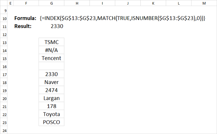
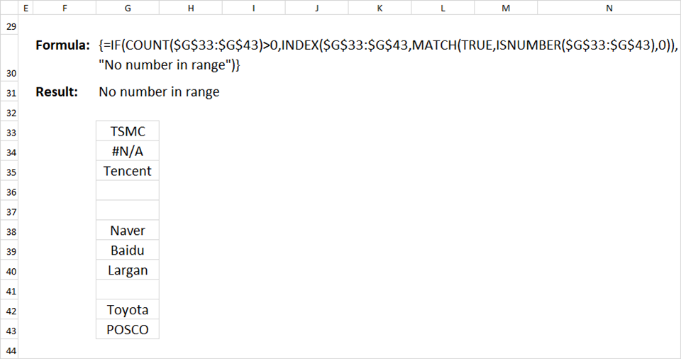
Another case is if any of the range that contains the weights has error or non-numerical values. Some scrubbing of the data beforehand or some error handling in the formula would be needed in this case.


Happy Sorting!

31 Dec 2019

How To Find Last Occurrence of Character in a String

There may be some instances where you will need to find the last occurrence of a specific character in a string in Excel. The following example shows you how.

Assuming that your original string is in cell B2 and the character that you want to find is "." , the formula to give you the position of the last occurrence of the character in the string is:
=LEN(B2)-LEN(TRIM(RIGHT(SUBSTITUTE(B2,".",REPT(" ",LEN(B2))),LEN(B2))))

The following shows a breakdown of the above formula:

The key to this example is this magical formula, which gives you everything to the right of the last occurrence of the character ".".
=TRIM(RIGHT(SUBSTITUTE(B2,".",REPT(" ",LEN(B2))),LEN(B2)))

This formula is useful if you want to find the extension of a filename (for example .xlsx or .docx) or the filename, folder name or worksheet name.

31 Oct 2019

How to find the first numerical value in a range

The following Excel formula will give you the first numerical value in a range (whether a row or column):

Conceptual Formula:

{=INDEX(RangeToSearch, MATCH(TRUE, ISNUMBER(RangeToSearch), 0)}

where RangeToSearch is a range such as $F$13:$P$13.

Example:

{=INDEX($F$13:$P$13, MATCH(TRUE, ISNUMBER($F$13:$P$13), 0))}

This formula works whether the range is a row or column. (but not for multiple rows/columns). It works even if there are #N/A or text values in the range.

However, the formula will give an #N/A if there is no number in the range. We can add error handling to the formula, with the following:

With error handling:

{=IF(COUNT(RangeToSearch)>0, INDEX(RangeToSearch, MATCH(TRUE, ISNUMBER(RangeToSearch),0)), ValueifError)

where ValueifError is the value if there are no numbers in the range. Count(RangeToSearch) counts the number of numerical values in the range RangeToSearch.

Example:

=IF(COUNT($F$23:$P$23)>0, INDEX($F$23:$P$23, MATCH(TRUE, ISNUMBER($F$23:$P$23), 0)), "No number in range")

Note: These are array formulas, so it must be entered using Shift-Ctrl-Enter.